💵The Gigantic Gender Pay Gap💵
Esther Mejia and Shailee Shah
Last updated on 2018-12-21
#load Packages here
library(tidyverse)
library(leaflet)
library(readr)
library(scales)
#reading the .cvs file
Census_data <- read_csv("acs2015_census_tract_data.csv")
Gender_occupation <- read_csv("inc_occ_gender.csv")
Gender_pay_gap <- read_csv("Gender_Pay_Gap.csv")

#data wrangling for the Census_data
#we want to the dataset to only include the information that we are going to work with
#this dataset will be used to show the gender pay gap in Northeastern States in a graph
Clean_Census_data <- Census_data %>%
  select(State,TotalPop, Men, Women) %>%
  filter(State %in% c("Maine", "Vermont", "New Hampshire", "Massachusetts", "New York","Rhode Island", "Connecticut","Pennsykvania", "New Jeresy")) %>%
  group_by(State) %>%
  summarize(sum_totalPop = sum(TotalPop), sum_men = sum(Men), sum_women = sum(Women))
#this census dataset is what we are going to join
Cleaner_Census_data<- Census_data %>%
  select(State, TotalPop, Men, Women) %>%
  group_by(State) %>%
  summarize(sum_totalPop = sum(TotalPop), sum_men = sum(Men), sum_women = sum(Women))
#remove 2 observations since they were not states
Joining_Census_data <-Cleaner_Census_data[-c(9,40), ]
#data wrangling for the Gender_pay_gap to join with joining_Census_data
Clean_gender_pay_gap <- Gender_pay_gap %>%
  group_by(State) %>%
  summarize(Men_Salary=mean(Men_Salary),Women_Salary=mean(Women_Salary)) %>%
  mutate(Total_salary = ((Men_Salary + Women_Salary)/2))

Cleaner_gender_pay_gap<- rbind(Clean_gender_pay_gap, data.frame(State = "Nationally", t(colMeans(Clean_gender_pay_gap[,-1]))))

Nationally <-Cleaner_gender_pay_gap %>%
  slice(51:51) %>%
  gather("Men_Salary", "Women_Salary", "Total_salary" ,key = "Gender" , value = "Salary") %>%
  mutate(Average_Salary = "60,309")

Nationally$Gender[Nationally$Gender == "Men_Salary"] <- "Men"
Nationally$Gender[Nationally$Gender == "Women_Salary"] <- "Women"
Nationally$Gender[Nationally$Gender == "Total_salary"] <- "Average"

#joining the two datasets
Census_Gender_pay_gap <-Joining_Census_data %>%
  left_join(Clean_gender_pay_gap, by = "State")

#Occupation data wrangling
female_representation_compensation <- Gender_occupation %>%
  filter(Occupation == "Registered nurses" | Occupation == "Elementary and middle school teachers" | Occupation == "Social workers" | Occupation == "lawyer" | Occupation == "Driver/sales workers and truck drivers" | Occupation == "Financial analysts" | Occupation == "Chief executives" | Occupation == "Software developers, applications and systems software" | Occupation == "General and operations managers" | Occupation == "Computer and information systems managers" | Occupation == "Physicians and surgeons" | Occupation == "Real estate brokers and sales agents" | Occupation == "Bakers")%>%
  mutate(female_rep_percentage = F_workers/ All_workers * 100)%>%
  mutate(female_yearly_salary = as.numeric(F_weekly) * 52) %>%
  mutate(male_yearly_salary = as.numeric(M_weekly) * 52)

# create dummy outlier variable
female_representation_compensation <- female_representation_compensation %>%
 mutate(outlier = ifelse(Occupation %in% c("Chief executives", "Computer and information systems managers"), "Yes", "No"))

#data wrangling for barplot to show sterotypical job for the females
stereotypical_female_jobs <- female_representation_compensation %>%
  filter(Occupation == "Registered nurses" | Occupation == "Elementary and middle school teachers" | Occupation == "Social workers") %>%
  select(-c("All_workers","All_weekly","M_workers","M_weekly","F_workers","F_weekly","female_rep_percentage","outlier")) %>%
  gather("male_yearly_salary", "female_yearly_salary",key = "Yearly_salary" , value = "Salary")

#data wrangling for barplot to show sterotypical job for the males
stereotypical_male_jobs <- female_representation_compensation %>%
  filter(Occupation == "General and operations managers" | Occupation == "Driver/sales workers and truck drivers" | Occupation == "Physicians and surgeons") %>%
  select(-c("All_workers","All_weekly","M_workers","M_weekly","F_workers","F_weekly","female_rep_percentage","outlier")) %>%
  gather("male_yearly_salary", "female_yearly_salary",key = "Yearly_salary" , value = "Salary")
Gender Pay Gap Causes
Unconscious Bias
Although the Equal Pay Act of 1963 prohibits salary discrimination based on gender, unconscious bias ensures that women earn less than men within the same exact occupations 1. Without explicit cognitive acknowledgement, our socialized unconscious bias favors male professionals, increasing their promotion rate as decided by their managers.
Even when a woman and a man have the same skills and amount of experience, the man will attain the higher salary. This unconscious bias unfolds in an experiment in which the participants were asked how much the candidates represented on the resume they reviewed should receive 2. All the resumes were the same, except one set contained a female name, while the other set contained a male name. Participants consistently ascribed higher salaries to the male candidates.
#data visualization
#scatterplot code
ggplot(stereotypical_female_jobs, aes(x = Occupation, y=Salary, fill= Yearly_salary))+
  geom_col(position = "dodge") +
  theme(panel.background = element_rect(fill = "white")) +
  scale_fill_manual(values = c("male_yearly_salary"= "blue" ,"female_yearly_salary" = "pink"),name = "Gender", labels = c("Women", "Men"))+
  labs(title = "Salaries among Stereotypically Female Occupations",x = "", y = "Yearly Salary") +
  scale_y_continuous(labels=dollar)+
  scale_x_discrete(breaks=c("Elementary and middle school teachers","Registered nurses","Social workers"),
  labels=c("Primary School Teachers", "Registered Nurses", "Social Workers"))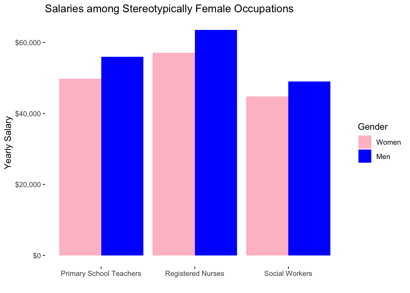
This unconscious bias even exists in occupations stereotypically for women, in which the majority of the workers are women. As demonstrated by the graph above, women earn less money than men across all represented professions sterotypically for women 3. These occupations are characterized in this way due to their inherent caring and nurturing nature. As demonstrated by the graph above, women earn less money than men across all represented professions stereotypically for women. This is surprising because all the women represented in these industries can advocate for higher wages for the betterment of their majority. However, managers exercise unconscious bias when distributing salaries by allocating slightly higher salaries to men for the same work as the women 4. Unfortunately, we are unaware of unconscious biases that instinctively determine our perceptions and choices.
Motherhood Penalty
This graph below reveals that occupations which are highly represented by women are correlated with lower salaries. The following randomly selected occupations are represented in the graph: elementary and middle school teachers, registered nurses, lawyers, truck drivers, financial analysts, software developers, general managers, computer managers, physicians and surgeons, real estate brokers and bakers. The outlier occupations have been highlighted to demonstrate that there are observations that deviate from the general pattern.
In general, women and men are segregated by occupation, with women outnumbering men in professions with lower salaries and fewer promotions 5. This can be attributed to the motherhood penalty, in which women make choices that benefit their children, but not their careers 6. Data from Britain suggests that 44-75 percent of mothers switch to a less demanding job and consequently a much lower pay in order to focus their time and energy on taking care of their children 7. As a result, women sacrifice their careers and potential for higher salaries in order to raise their children. Although fathers are engaging in more childcare than father from previous generations, women are significantly taking on the second shift- the additional responsibility of domestic chores along with work in the professional sector 8.
faves <- subset (female_representation_compensation, Occupation %in% c("Chief executives", "Driver/sales workers and truck drivers", "Bakers"))
ggplot(data = female_representation_compensation,
       mapping = aes(x = female_rep_percentage , y = as.numeric(female_yearly_salary))) +
  geom_point()+
  geom_smooth(method='lm',formula=y~x) + geom_point(data = faves, color = "red") + geom_text(aes(label = ifelse(Occupation %in% c("Chief executives",    "Driver/sales workers and truck drivers", "Bakers"), as.character(Occupation), " ")), hjust = 0, vjust = 0) +
  labs(title = "Variation between Salary and Female Representation by Occupation",x = "Female Representation by Occupation  (%)", y = "Female Yearly Salary")+
  scale_y_continuous(labels=dollar)+
theme(panel.background = element_rect(fill = "white")) 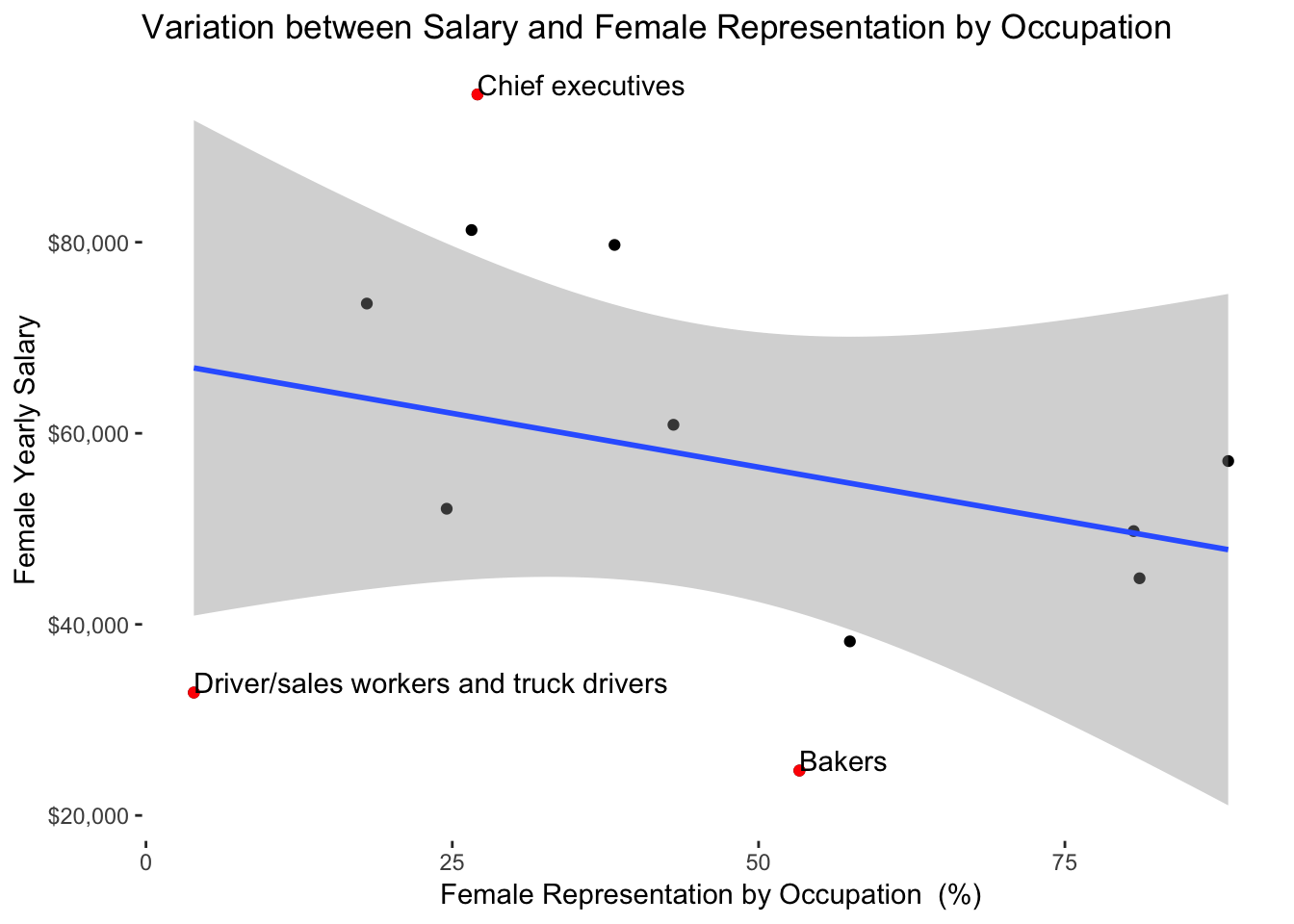
Solution
Bridging the Gender Pay Gap through Advocates within the Legal System
This graph reveals a negative correlation between the total population of women and the earning ratio of an average woman’s salary to an average man’s salary in Northeastern U.S. States to suggest that women in large numbers do not advocate for themselves to receive higher pays. There are many possible solutions to combat the gender pay gap, but mobilizing the masses will not close the gender pay gap. For example, during the national women’s marches in the beginning of January of 2017 and 2018, women zealously came together to advocate for their equity; however, there were not any tangible consequences that improved the plight of women. One march participant even stated, “So maybe there’s not an official change in government, but I do think that women feeling empowered is a really important part of our march of equality” 9.
According to the American Association of University Women, closing the gender pay gap will take action from individuals and policy makers. Instead of social movements for the masses, the gender pay gap should be reformed by individual advocates within the legal system. For example, in 1998, the equal pay activist Lily Ledbetter filed a discrimination lawsuit because the other male managers in her department were making twice as much as her. Her efforts resulted in the Lily Ledbetter Fair Pay Act of 2009, the first bill that President Obama signed into law. According to this law, a citizen could present an equal pay lawsuit from the date that the employer delivers the initial discriminatory wage, not at the date of the most recent pay check 10. This allowed for more gender pay gap cases within the legal system to actually begin to close this disparity through political forces.
Population_ratio_graph <- Census_Gender_pay_gap %>%
 filter(State == "Maine" | State == "Vermont"| State == "Massachusetts" | State == "Rhode Island" | State == "Connecticut" | State == "Pennsylvania" | State == "New Jersey") %>%
 mutate(ratio_women_salary = Women_Salary/ Men_Salary)

ggplot(data = Population_ratio_graph,
      mapping = aes(x = sum_women, y = ratio_women_salary)) +
 geom_point(color = "dark green", size = 2) +
  labs(title = "Relationship between Women's Population and Gender Pay Gap  ",x = "Total Population of Women", y = "Avg. Earnings Ratio (Avg. Women's Salary/ Avg. Men's Salary") +
 #geom_smooth(method='lm',formula=y~x) +
 scale_x_continuous(labels = scales :: comma) +
 scale_y_continuous(name = "Average Earnings Ratio", labels = scales:: percent) +
 geom_text(aes(label = ifelse(sum_women < 6000000, as.character(State), ""), hjust = 0, vjust = -0.5))+
 geom_text(aes(label = ifelse(sum_women > 6000000, as.character(State), ""), hjust = 1, vjust = -0.5))+
 theme(panel.background = element_rect(fill = "white", color = "grey50"))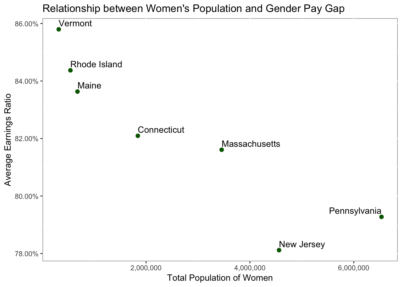
“Why does the gender wage gap still exist?” CNN, www.cnn.com/videos/cnnmoney/2018/04/10/why-does-teh-wage-gap-still-exist.cnn/video/playlists/womens-issues-worldwide/.↩
Elsesser, Kim. “Unequal Pay, Unconscious Bias, And What To Do About It.” Forbes, 10 Apr. 2018.↩
“The gender pay gap.” The Economist, 7 Oct. 2017, www.economist.com/international/2017/10/07/the-gender-pay-gap.↩
“Why does the gender wage gap still exist?” CNN, www.cnn.com/videos/cnnmoney/2018/04/10/why-does-teh-wage-gap-still-exist.cnn/video/playlists/womens-issues-worldwide/.↩
“The gender pay gap.” The Economist, 7 Oct. 2017, www.economist.com/international/2017/10/07/the-gender-pay-gap.↩
“Why does the gender wage gap still exist?” CNN, www.cnn.com/videos/cnnmoney/2018/04/10/why-does-teh-wage-gap-still-exist.cnn/video/playlists/womens-issues-worldwide/.↩
“The gender pay gap.” The Economist, 7 Oct. 2017, www.economist.com/international/2017/10/07/the-gender-pay-gap.↩
Wong, Kristin. “There’s a Stress Gap Between Men and Women. Here’s Why It’s Important.” The New York Times, www.nytimes.com/2018/11/14/smarter-living/stress-gap-women-men.html?fallback=0&recId=1Dy9Za86kEczXml2L8ha45st9mi&locked=0&geoContinent=NA&geoRegion=MA&recAlloc=contextual-bandit-home-geo&geoCountry=US&blockId=home-living-vi&imp_id=398125922&action=click&module=Smarter%20Living&pgtype=Homepage.↩
Wright, Katie. “Women’s March: What’s changed one year on?” BBC News, 21 Jan. 2018, www.bbc.com/news/uk-42767434.↩
“LEDBETTER v. GOODYEAR TIRE & RUBBER CO. (No. 05-1074) 421 F. 3d 1169, affirmed.” Cornell University Law School, www.law.cornell.edu/supct/html/05-1074.ZS.html.↩